Temperature Attribution Analysis

3.7. Temperature Attribution Analysis#

Decomposing temperature changes into physically meaningful components.

When comparing SUEWS simulations, you can easily see that T2 (2m air temperature) differs between scenarios. But this doesn’t tell you why. The attribution module answers these questions by decomposing temperature differences using Shapley value analysis [Owen, 1972, Shapley, 1953] – a mathematically exact method that guarantees the sum of contributions equals the total change.

This tutorial demonstrates:

Single-run diagnostics – detect and attribute T2 anomalies
Two-scenario comparison – decompose the temperature difference from a green-infrastructure intervention
Flux budget breakdown – identify which energy balance component drives the change

Prerequisites: Complete SUEWS Quick Start Tutorial first.

API approach: This tutorial uses the SUEWSSimulation OOP interface but extracts DataFrames for scenario comparison. This hybrid pattern is appropriate for attribution studies where output DataFrames from two runs must be compared.

3.7.1. Setup#

import matplotlib.pyplot as plt
import pandas as pd

from supy import SUEWSSimulation
from supy.util import attribute_t2, diagnose_t2

3.7.2. Load Sample Data and Run Baseline Simulation#

Load the built-in sample dataset and slice to a summer period. Drop the first row with .iloc[1:] because accumulated variables (e.g. rainfall) for the partial period at the slice boundary are incomplete, making that row invalid as forcing input.

sim_baseline = SUEWSSimulation.from_sample_data()

# Use a shorter period for demonstration
df_forcing = sim_baseline.forcing["2012-06":"2012-08"].iloc[1:]
sim_baseline.update_forcing(df_forcing)

# Run baseline simulation
df_output_baseline = sim_baseline.run()

print(f"Simulation period: {df_forcing.index[0]} to {df_forcing.index[-1]}")
print(f"Number of timesteps: {len(df_forcing)}")
print("\nForcing variables available: Tair, RH, pres (needed for attribution)")

Simulation period: 2012-06-01 00:05:00 to 2012-08-31 23:55:00
Number of timesteps: 26495

Forcing variables available: Tair, RH, pres (needed for attribution)

3.7.3. Use Case 1: Diagnosing Unexpected T2 Values#

A common question when running SUEWS is: “Why does T2 behave unexpectedly at certain times?” The diagnose_t2() function automatically identifies anomalous timesteps and attributes the causes.

3.7.3.1. Quick Anomaly Detection#

Detect timesteps where T2 exceeds 2 standard deviations from the daily mean. Passing df_forcing enables accurate attribution of air-property contributions.

result_anomaly = diagnose_t2(
    df_output_baseline,
    df_forcing=df_forcing,
    method="anomaly",
    threshold=2.0,
    hierarchical=True,
)

print(result_anomaly)

T2 Attribution Results
========================================
Mean delta_T2: +0.352 degC

Component Breakdown:
----------------------------------------
  T_ref          : -0.249 degC (-70.7%)
  flux_total     : +0.484 degC (137.6%)
  resistance     : +0.112 degC ( 31.9%)
  air_props      : +0.004 degC (  1.2%)

  Flux breakdown:
      dQstar     : +0.986 degC (280.4%)
      dQE        : -0.048 degC (-13.6%)
      ddQS       : -0.569 degC (-161.9%)
      dQF        : +0.115 degC ( 32.8%)

Closure residual: 0.00e+00 degC

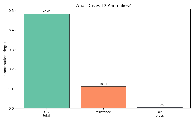
3.7.3.2. Interpreting the Results#

The output shows three top-level contributions:

flux_total – sensible heat flux changes
resistance – turbulent exchange efficiency
air_props – air density and heat capacity

If flux dominates, investigate the energy balance components. If resistance dominates, check wind speed and stability conditions.

fig, ax = plt.subplots(figsize=(8, 5))
result_anomaly.plot(kind="bar", ax=ax)
ax.set_title("What Drives T2 Anomalies?")
plt.tight_layout()

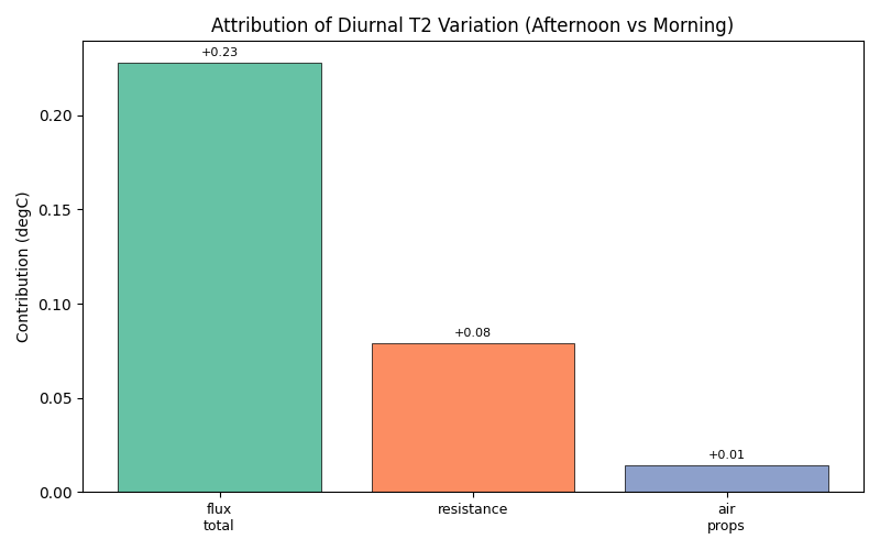
3.7.3.3. Diurnal Cycle Analysis#

Compare afternoon peak vs. morning baseline to understand the diurnal temperature pattern:

result_diurnal = diagnose_t2(
    df_output_baseline,
    df_forcing=df_forcing,
    method="diurnal",
    hierarchical=True,
)

print("Diurnal T2 Attribution:")
print(result_diurnal)

Diurnal T2 Attribution:
T2 Attribution Results
========================================
Mean delta_T2: +3.110 degC

Component Breakdown:
----------------------------------------
  T_ref          : +2.789 degC ( 89.7%)
  flux_total     : +0.228 degC (  7.3%)
  resistance     : +0.079 degC (  2.5%)
  air_props      : +0.014 degC (  0.5%)

  Flux breakdown:
      dQstar     : +0.482 degC ( 15.5%)
      dQE        : -0.160 degC ( -5.2%)
      ddQS       : -0.247 degC ( -7.9%)
      dQF        : +0.153 degC (  4.9%)

Closure residual: 0.00e+00 degC

The diurnal method returns an aggregate comparison (afternoon 12–15 h vs morning 6–10 h), so kind='bar' shows the mean contributions.

fig, ax = plt.subplots(figsize=(8, 5))
result_diurnal.plot(kind="bar", ax=ax)
ax.set_title("Attribution of Diurnal T2 Variation (Afternoon vs Morning)")
plt.tight_layout()

Attribution of Diurnal T2 Variation (Afternoon vs Morning)

3.7.4. Use Case 2: Green Infrastructure Impact Attribution#

A fundamental question in urban climate research: when we add vegetation, which physical mechanisms drive the temperature reduction?

We compare two scenarios:

Baseline – higher building/paved fraction
Green – increased vegetation fraction

sim_green = SUEWSSimulation.from_sample_data()
sim_green.update_forcing(df_forcing)

# Access the land cover configuration
lc = sim_green.config.sites[0].properties.land_cover
surface_types = ["paved", "bldgs", "evetr", "dectr", "grass", "bsoil", "water"]

print("Current surface fractions:")
for name in surface_types:
    print(f"  {name}: {getattr(lc, name).sfr}")

Current surface fractions:
  paved: 0.43
  bldgs: 0.38
  evetr: 0.0
  dectr: 0.02
  grass: 0.03
  bsoil: 0.0
  water: 0.14

3.7.4.1. Modify Surface Fractions#

Use update_config with a dictionary that mirrors the YAML structure. This is the recommended approach for parameter changes – it keeps the interaction at the configuration level rather than exposing internal DataFrames.

Reduce paved fraction by 0.15 and increase grass by 0.15.

sim_green.update_config(
    {
        "sites": {
            "properties": {
                "land_cover": {
                    "paved": {"sfr": lc.paved.sfr.value - 0.15},
                    "grass": {"sfr": lc.grass.sfr.value + 0.15},
                }
            }
        }
    }
)

print("Modified surface fractions:")
for name in surface_types:
    print(f"  {name}: {getattr(lc, name).sfr}")

Modified surface fractions:
  paved: 0.28
  bldgs: 0.38
  evetr: 0.0
  dectr: 0.02
  grass: 0.18
  bsoil: 0.0
  water: 0.14

3.7.4.2. Run Greened Scenario#

df_output_green = sim_green.run()

print("Both scenarios simulated successfully")

Both scenarios simulated successfully

3.7.4.3. Traditional Comparison: What Changed?#

Extract T2 from both scenarios and compute the difference. This tells us what changed but not why.

def get_t2(output):
    """Extract T2 series from SUEWSOutput."""
    return output.get_variable("T2", group="SUEWS").iloc[:, 0]


t2_baseline = get_t2(df_output_baseline)
t2_green = get_t2(df_output_green)
delta_t2 = t2_green - t2_baseline

print(f"Mean T2 change: {delta_t2.mean():.2f} degC")
print(f"Max cooling: {delta_t2.min():.2f} degC")
print(f"Max warming: {delta_t2.max():.2f} degC")

Mean T2 change: -0.10 degC
Max cooling: -0.43 degC
Max warming: 0.45 degC

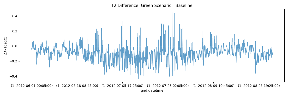
Plot the raw temperature difference time series.

fig, ax = plt.subplots(figsize=(12, 4))
delta_t2.plot(ax=ax, alpha=0.7)
ax.axhline(0, color="black", linestyle="--", linewidth=0.5)
ax.set_ylabel(r"$\Delta T_2$ (degC)")
ax.set_title("T2 Difference: Green Scenario - Baseline")
plt.tight_layout()

T2 Difference: Green Scenario - Baseline

3.7.4.4. Attribution Analysis: Why Did It Change?#

Now use attribute_t2() to decompose the temperature difference into physically meaningful contributions. Both scenarios share the same forcing, so we pass df_forcing for both.

result_green = attribute_t2(
    df_output_A=df_output_baseline,
    df_output_B=df_output_green,
    df_forcing_A=df_forcing,
    df_forcing_B=df_forcing,
    hierarchical=True,
)

print(result_green)

T2 Attribution Results
========================================
Mean delta_T2: -0.098 degC

Component Breakdown:
----------------------------------------
  T_ref          : +0.000 degC ( -0.0%)
  flux_total     : -0.156 degC (159.6%)
  resistance     : +0.058 degC (-59.7%)
  air_props      : +0.000 degC ( -0.0%)

  Flux breakdown:
      dQstar     : -0.020 degC ( 20.5%)
      dQE        : -0.169 degC (173.7%)
      ddQS       : +0.033 degC (-33.6%)
      dQF        : +0.001 degC ( -0.9%)

Closure residual: -3.03e-05 degC

3.7.4.5. Visualise the Attribution#

The bar chart (left) shows mean contributions from each mechanism; the diurnal plot (right) reveals how they vary through the day.

fig, axes = plt.subplots(1, 2, figsize=(14, 5))

result_green.plot(kind="bar", ax=axes[0])
axes[0].set_title(r"Attribution of $\Delta T_2$ to Physical Mechanisms")

result_green.plot(kind="diurnal", ax=axes[1])
axes[1].set_title("Diurnal Pattern of Attribution Components")

plt.tight_layout()

$Attribution of $\Delta T_2$ to Physical Mechanisms, Diurnal Pattern of Attribution Components$

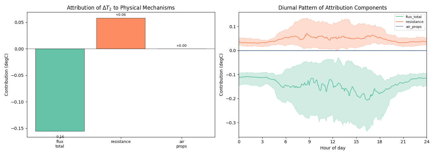
3.7.4.6. Flux Budget Breakdown#

With hierarchical=True, you can see how much each energy balance component contributes:

flux_cols = [
    c
    for c in result_green.contributions.columns
    if c.startswith("flux_") and c != "flux_total"
]

if flux_cols:
    fig, ax = plt.subplots(figsize=(10, 5))
    result_green.plot(kind="bar", ax=ax, components=flux_cols)
    ax.set_title("Flux Budget Breakdown: Which Energy Balance Component Matters Most?")
    plt.tight_layout()
else:
    print("Flux breakdown not available - run with hierarchical=True")

Flux Budget Breakdown: Which Energy Balance Component Matters Most?

3.7.5. Summary#

This tutorial demonstrated how to decompose temperature changes into physically meaningful components:

Single-run diagnostics with diagnose_t2() – detect anomalous timesteps and attribute them to flux, resistance, or air-property contributions
Two-scenario comparison with attribute_t2() – decompose the temperature difference between a baseline and a green-infrastructure scenario
Flux budget breakdown – identify whether radiation, evaporation, storage, or anthropogenic heat drives the change

Both functions return an AttributionResult object with:

.contributions – full timeseries of each component
.summary – summary statistics (mean, std, min, max)
.plot() – built-in visualisation (bar, diurnal, line, heatmap)
print() – clean text summary with percentages

Practical applications:

Urban planning – understand why green infrastructure works, not just that it works
Model debugging – identify which process causes unexpected behaviour
Sensitivity analysis – quantify the relative importance of different physical processes
Climate adaptation – design interventions that target the most effective mechanisms

Next steps:

Impact Studies Using SuPy – sensitivity analysis across scenarios
Analysing Simulation Results – validation and export of results

Total running time of the script: (0 minutes 41.254 seconds)

Gallery generated by Sphinx-Gallery