Tip

1. Need help? Please let us know in the SUEWS Community.

2. Please report issues with the manual on GitHub Issues (or use Report Issue for This Page for page-specific feedback).

3. Please cite SUEWS with proper information from our Zenodo page.

3.5. Analysing Simulation Results

Comprehensive analysis and validation of SUEWS outputs.

Understanding and analysing SUEWS output is essential for scientific interpretation and model validation. This tutorial covers:

1. Output structure - Navigating the results DataFrame

2. Statistical analysis - Energy and water balance calculations

3. Diagnostic plots - Visualising model behaviour

4. Validation - Comparing with observations

5. Export - Saving results for further use

Prerequisites: Complete SUEWS Quick Start Tutorial first.

import matplotlib.pyplot as plt
import numpy as np
import pandas as pd
from scipy import stats

from supy import SUEWSSimulation

3.5.1. Load and Run Simulation

First, run a simulation to generate results for analysis.

sim = SUEWSSimulation.from_sample_data()
output = sim.run()

print("Simulation complete!")
print(f"Output period: {output.times[0]} to {output.times[-1]}")
print(f"Time steps: {len(output.times)}")

Simulation complete!
Output period: 2012-01-01 00:05:00 to 2013-01-01 00:00:00
Time steps: 105408

3.5.2. Understanding Output Structure

SUEWS results use MultiIndex columns organised by output groups:

• SUEWS: Primary energy and water balance (QN, QH, QE, QS, QF, etc.)

• DailyState: Daily summary variables (LAI, GDD, snow density)

• snow: Detailed snow variables by surface type

• RSL: Roughness sublayer profiles

Access variables using get_variable() or direct MultiIndex indexing.

results = output.df

# Method 1: get_variable() on output object - recommended
qh = output.get_variable("QH", group="SUEWS")
print(f"QH shape: {qh.shape}")

# Method 2: Direct MultiIndex access on raw DataFrame
qn = results[("SUEWS", "QN")]
print(f"QN shape: {qn.shape}")

# List available groups and variables
print(f"\nAvailable groups: {output.groups}")
print(f"SUEWS variables (first 10): {results['SUEWS'].columns.tolist()[:10]}")

QH shape: (105408, 1)
QN shape: (105408,)

Available groups: ['SUEWS', 'snow', 'BEERS', 'ESTM', 'EHC', 'DailyState', 'RSL', 'debug', 'SPARTACUS', 'STEBBS', 'NHood']
SUEWS variables (first 10): ['Kdown', 'Kup', 'Ldown', 'Lup', 'Tsurf', 'QN', 'QF', 'QS', 'QH', 'QE']

3.5.3. Helper Function for Variable Access

Create a helper to simplify extracting multiple variables.

def get_var(out, name, group="SUEWS"):
    """Extract a single variable as a Series with DatetimeIndex.

    Assumes single-grid output (as produced by the sample data).
    Raises an error if multiple grids are present, since dropping
    the grid level would produce a non-unique index.
    """
    ser = out.get_variable(name, group=group).iloc[:, 0]
    # Drop grid level only when safe (single grid)
    if isinstance(ser.index, pd.MultiIndex) and ser.index.nlevels == 2:
        n_grids = ser.index.get_level_values("grid").nunique()
        if n_grids != 1:
            raise ValueError(
                f"Expected single-grid output, but found {n_grids} grids. "
                "Use MultiIndex indexing directly for multi-grid runs."
            )
        ser = ser.droplevel("grid")
    return ser


def get_vars(out, names, group="SUEWS"):
    """Extract multiple variables as a DataFrame with DatetimeIndex."""
    return pd.DataFrame({name: get_var(out, name, group) for name in names})


# Extract energy balance components
energy_vars = ["QN", "QF", "QS", "QE", "QH"]
energy_df = get_vars(output, energy_vars)

print("Energy balance components:")
print(energy_df.head())

Energy balance components:
                            QN         QF         QS         QE         QH
datetime
2012-01-01 00:05:00 -27.368506  56.837839 -50.460870  11.202703  68.727500
2012-01-01 00:10:00 -27.368506  55.647518 -50.274281  11.084424  67.468869
2012-01-01 00:15:00 -27.368506  54.457197 -50.102896  10.967406  66.224181
2012-01-01 00:20:00 -27.368506  53.266875 -49.871668  10.845190  64.924847
2012-01-01 00:25:00 -27.368506  52.076554 -49.668152  10.725328  63.650872

3.5.4. Basic Statistics

Calculate summary statistics for the energy balance.

print("Annual Energy Balance Statistics (W/m2):")
print(energy_df.describe().round(1))

# Seasonal means using meteorological seasons (month-based grouping)
season_map = {12: "Winter (DJF)", 1: "Winter (DJF)", 2: "Winter (DJF)",
              3: "Spring (MAM)", 4: "Spring (MAM)", 5: "Spring (MAM)",
              6: "Summer (JJA)", 7: "Summer (JJA)", 8: "Summer (JJA)",
              9: "Autumn (SON)", 10: "Autumn (SON)", 11: "Autumn (SON)"}
season_order = ["Winter (DJF)", "Spring (MAM)", "Summer (JJA)", "Autumn (SON)"]
seasonal = energy_df.groupby(energy_df.index.month.map(season_map)).mean()
seasonal = seasonal.loc[[s for s in season_order if s in seasonal.index]]
print("\nSeasonal Means (W/m2):")
print(seasonal.round(1))

Annual Energy Balance Statistics (W/m2):
             QN        QF        QS        QE        QH
count  105408.0  105408.0  105408.0  105408.0  105408.0
mean       44.8      84.5      12.9      27.6      88.8
std       138.7      32.8      82.9      23.1      67.1
min       -84.5      31.1     -83.9       1.6     -43.4
25%       -41.5      53.6     -45.3      11.6      40.9
50%       -24.9      88.0     -15.9      19.7      69.3
75%        81.0     112.7      35.2      37.3     124.8
max       721.4     161.3     402.9     241.2     365.5

Seasonal Means (W/m2):
                 QN    QF    QS    QE     QH
datetime
Winter (DJF)  -14.4  92.6   1.6  16.7   60.0
Spring (MAM)   69.9  85.5  31.8  28.1   95.5
Summer (JJA)  100.4  77.0  27.0  39.0  111.3
Autumn (SON)   22.2  83.2  -9.0  26.4   88.0

3.5.5. Energy Balance Closure

Verify that the energy balance closes: QN + QF = QS + QE + QH

energy_in = get_var(output, "QN") + get_var(output, "QF")
energy_out = get_var(output, "QS") + get_var(output, "QE") + get_var(output, "QH")
residual = energy_in - energy_out

print("Energy Balance Closure Check:")
print(f"  Mean residual: {residual.mean():.4f} W/m2")
print(f"  Std residual:  {residual.std():.4f} W/m2")
print(f"  Max |residual|: {residual.abs().max():.4f} W/m2")
print("\nNote: SUEWS enforces closure by design. Non-zero residuals")
print("indicate numerical precision limits only.")

Energy Balance Closure Check:
  Mean residual: -0.0000 W/m2
  Std residual:  0.0000 W/m2
  Max |residual|: 0.0000 W/m2

Note: SUEWS enforces closure by design. Non-zero residuals
indicate numerical precision limits only.

3.5.6. Water Balance Analysis

Calculate annual water balance: P + I = E + R + D + dS

rain = get_var(output, "Rain")
evap = get_var(output, "Evap")
runoff = get_var(output, "RO")
drainage = get_var(output, "Drainage")
irr = get_var(output, "Irr")
storage_change = get_var(output, "TotCh")

# Annual totals (mm/year)
print("Annual Water Balance (mm):")
print("  Inputs:")
print(f"    Precipitation: {rain.sum():.1f}")
print(f"    Irrigation:    {irr.sum():.1f}")
print("  Outputs:")
print(f"    Evaporation:   {evap.sum():.1f}")
print(f"    Runoff:        {runoff.sum():.1f}")
print(f"    Drainage:      {drainage.sum():.1f}")
print(f"  Storage change:  {storage_change.sum():.1f}")

water_residual = (rain.sum() + irr.sum()) - evap.sum() - runoff.sum() - drainage.sum() - storage_change.sum()
print(f"  Residual:        {water_residual:.1f}")

Annual Water Balance (mm):
  Inputs:
    Precipitation: 821.0
    Irrigation:    0.0
  Outputs:
    Evaporation:   352.2
    Runoff:        573.9
    Drainage:      725.5
  Storage change:  -105.1
  Residual:        -725.5

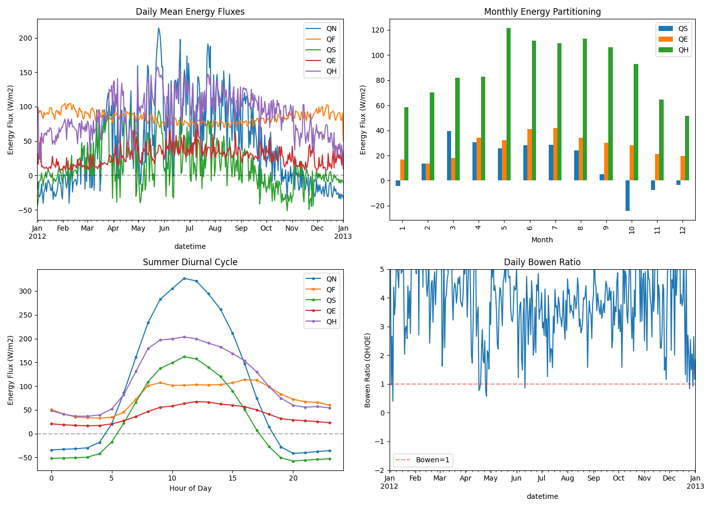
3.5.7. Energy Balance Time Series

Visualise energy fluxes over time.

fig, axes = plt.subplots(2, 2, figsize=(14, 10))

# 1. Daily energy fluxes
ax = axes[0, 0]
daily_energy = energy_df.resample("D").mean()
daily_energy.plot(ax=ax)
ax.set_ylabel("Energy Flux (W/m2)")
ax.set_title("Daily Mean Energy Fluxes")
ax.legend(loc="upper right")
ax.axhline(y=0, color="k", linestyle="--", alpha=0.3)

# 2. Monthly energy partitioning
ax = axes[0, 1]
monthly_means = energy_df[["QS", "QE", "QH"]].groupby(energy_df.index.month).mean()
monthly_means.plot(kind="bar", ax=ax)
ax.set_xlabel("Month")
ax.set_ylabel("Energy Flux (W/m2)")
ax.set_title("Monthly Energy Partitioning")
ax.legend(loc="upper right")

# 3. Diurnal cycle (summer if available, otherwise all data)
ax = axes[1, 0]
summer_mask = energy_df.index.month.isin([6, 7, 8])
if summer_mask.any():
    diurnal_energy = energy_df[summer_mask]
    diurnal_label = "Summer Diurnal Cycle"
else:
    diurnal_energy = energy_df
    diurnal_label = "Diurnal Cycle (all available data)"
hourly_diurnal = diurnal_energy.groupby(diurnal_energy.index.hour).mean()
hourly_diurnal.plot(ax=ax, marker="o", markersize=3)
ax.set_xlabel("Hour of Day")
ax.set_ylabel("Energy Flux (W/m2)")
ax.set_title(diurnal_label)
ax.legend(loc="upper right")
ax.axhline(y=0, color="k", linestyle="--", alpha=0.3)

# 4. Bowen ratio (QH/QE) over time
ax = axes[1, 1]
bowen = get_var(output, "QH") / get_var(output, "QE").replace(0, np.nan)
bowen_daily = bowen.resample("D").mean()
bowen_daily.plot(ax=ax)
ax.set_ylabel("Bowen Ratio (QH/QE)")
ax.set_title("Daily Bowen Ratio")
ax.set_ylim(-2, 5)
ax.axhline(y=1, color="r", linestyle="--", alpha=0.5, label="Bowen=1")
ax.legend()

plt.tight_layout()

3.5.8. Temperature Analysis

Analyse air and surface temperature patterns.

t2 = get_var(output, "T2")
tsurf = get_var(output, "Tsurf")

fig, axes = plt.subplots(2, 2, figsize=(14, 10))

# 1. Temperature time series
ax = axes[0, 0]
t2.resample("D").mean().plot(ax=ax, label="T2 (2m air)")
tsurf.resample("D").mean().plot(ax=ax, label="Tsurf (surface)")
ax.set_ylabel("Temperature (degC)")
ax.set_title("Daily Mean Temperatures")
ax.legend()

# 2. Temperature distribution
ax = axes[0, 1]
ax.hist(t2.dropna(), bins=50, alpha=0.7, label="T2", density=True)
ax.hist(tsurf.dropna(), bins=50, alpha=0.7, label="Tsurf", density=True)
ax.set_xlabel("Temperature (degC)")
ax.set_ylabel("Density")
ax.set_title("Temperature Distribution")
ax.legend()

# 3. Diurnal temperature cycle by season
ax = axes[1, 0]
for season_name, months in [
    ("Winter", [12, 1, 2]),
    ("Spring", [3, 4, 5]),
    ("Summer", [6, 7, 8]),
    ("Autumn", [9, 10, 11]),
]:
    mask = t2.index.month.isin(months)
    if not mask.any():
        continue
    hourly = t2[mask].groupby(t2[mask].index.hour).mean()
    ax.plot(hourly.index, hourly.values, marker="o", markersize=3, label=season_name)
ax.set_xlabel("Hour of Day")
ax.set_ylabel("T2 (degC)")
ax.set_title("Seasonal Diurnal Temperature Cycles")
ax.legend()

# 4. Surface-air temperature difference
ax = axes[1, 1]
delta_t = tsurf - t2
delta_t_hourly = delta_t.groupby(delta_t.index.hour).mean()
ax.plot(delta_t_hourly.index, delta_t_hourly.values, "ko-")
ax.set_xlabel("Hour of Day")
ax.set_ylabel("Tsurf - T2 (degC)")
ax.set_title("Surface-Air Temperature Difference")
ax.axhline(y=0, color="r", linestyle="--", alpha=0.5)
ax.fill_between(delta_t_hourly.index, 0, delta_t_hourly.values, where=delta_t_hourly.values > 0, alpha=0.3, color="red", label="Surface warmer")
ax.fill_between(delta_t_hourly.index, 0, delta_t_hourly.values, where=delta_t_hourly.values < 0, alpha=0.3, color="blue", label="Air warmer")
ax.legend()

plt.tight_layout()

3.5.9. Validation Statistics

Calculate standard validation metrics for model-observation comparison.

def validation_statistics(observed, modelled):
    """Calculate validation statistics.

    Parameters
    ----------
    observed : Series
        Observed values
    modelled : Series
        Modelled values (aligned with observed)

    Returns
    -------
    dict
        Validation statistics including bias, RMSE, R2, and IoA
    """
    # Align data
    obs, mod = observed.align(modelled, join="inner")
    obs = obs.dropna()
    mod = mod.loc[obs.index].dropna()

    # Re-align after dropna
    obs, mod = obs.align(mod, join="inner")

    n = len(obs)
    if n < 3:
        return {"n": n, "error": "Insufficient data"}

    mean_obs = obs.mean()
    mean_mod = mod.mean()

    # Bias
    bias = mean_mod - mean_obs

    # RMSE
    rmse = np.sqrt(((mod - obs) ** 2).mean())

    # Correlation
    r, p = stats.pearsonr(obs, mod)

    # Mean Absolute Error
    mae = (mod - obs).abs().mean()

    # Index of Agreement d1 (Willmott, 1981, doi:10.1080/02723646.1981.10642213)
    numer = ((mod - obs) ** 2).sum()
    denom_terms = ((mod - mean_obs).abs() + (obs - mean_obs).abs()) ** 2
    ioa = 1 - numer / denom_terms.sum() if denom_terms.sum() > 0 else np.nan

    return {
        "n": n,
        "mean_obs": mean_obs,
        "mean_mod": mean_mod,
        "bias": bias,
        "rmse": rmse,
        "mae": mae,
        "r": r,
        "r2": r**2,
        "p_value": p,
        "ioa": ioa,
    }


# Example: Compare modelled T2 with forcing Tair (as proxy for "observations")
# In practice, you would load actual observation data
tair_forcing = sim.forcing.df["Tair"]
t2_model = get_var(output, "T2")

stats_t2 = validation_statistics(tair_forcing, t2_model)
print("T2 vs Forcing Tair (demonstration):")
for key, val in stats_t2.items():
    if isinstance(val, float):
        print(f"  {key}: {val:.3f}")
    else:
        print(f"  {key}: {val}")

T2 vs Forcing Tair (demonstration):
  n: 105408
  mean_obs: 11.106
  mean_mod: 11.914
  bias: 0.808
  rmse: 0.991
  mae: 0.811
  r: 0.996
  r2: 0.993
  p_value: 0.000
  ioa: 0.993

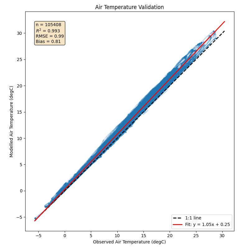
3.5.10. Validation Scatter Plot

Create a scatter plot comparing model output with observations.

def validation_scatter(observed, modelled, variable_name, units="", ax=None):
    """Create validation scatter plot with statistics."""
    if ax is None:
        fig, ax = plt.subplots(figsize=(8, 8))

    obs, mod = observed.align(modelled, join="inner")
    obs = obs.dropna()
    mod = mod.loc[obs.index].dropna()
    obs, mod = obs.align(mod, join="inner")

    ax.scatter(obs, mod, alpha=0.1, s=5)

    # 1:1 line
    lims = [min(obs.min(), mod.min()), max(obs.max(), mod.max())]
    ax.plot(lims, lims, "k--", label="1:1 line", linewidth=2)

    # Regression line
    slope, intercept = np.polyfit(obs, mod, 1)
    ax.plot(lims, [slope * x + intercept for x in lims], "r-", label=f"Fit: y = {slope:.2f}x + {intercept:.2f}", linewidth=2)

    # Statistics annotation
    stats_dict = validation_statistics(observed, modelled)
    stats_text = f"n = {stats_dict['n']}\n" f"$R^2$ = {stats_dict['r2']:.3f}\n" f"RMSE = {stats_dict['rmse']:.2f}\n" f"Bias = {stats_dict['bias']:.2f}"
    ax.text(0.05, 0.95, stats_text, transform=ax.transAxes, verticalalignment="top", fontsize=10, bbox=dict(boxstyle="round", facecolor="wheat", alpha=0.8))

    ax.set_xlabel(f"Observed {variable_name} ({units})")
    ax.set_ylabel(f"Modelled {variable_name} ({units})")
    ax.set_title(f"{variable_name} Validation")
    ax.legend(loc="lower right")
    ax.set_aspect("equal", adjustable="box")

    return ax


fig, ax = plt.subplots(figsize=(8, 8))
validation_scatter(tair_forcing, t2_model, "Air Temperature", "degC", ax=ax)
plt.tight_layout()

3.5.11. Exporting Results

Save results in various formats for further analysis.

# Export to CSV
export_vars = ["QN", "QH", "QE", "QS", "T2", "RH2"]
export_df = get_vars(output, export_vars)
# export_df.to_csv('suews_output.csv')  # Uncomment to save
print(f"Export DataFrame shape: {export_df.shape}")
print(f"Ready to save with: export_df.to_csv('suews_output.csv')")

# Export final state for restart runs
final_state = sim.state_final
# final_state.to_csv('final_state.csv')  # Uncomment to save
print(f"\nFinal state shape: {final_state.shape}")
print("Ready to save with: final_state.to_csv('final_state.csv')")

Export DataFrame shape: (105408, 6)
Ready to save with: export_df.to_csv('suews_output.csv')

Final state shape: (1, 2287)
Ready to save with: final_state.to_csv('final_state.csv')

3.5.12. Summary

Key analysis techniques covered:

1. Access variables with get_variable() or MultiIndex indexing

2. Check balance closure - energy and water budgets should close

3. Seasonal patterns - use groupby() with month/quarter

4. Diurnal patterns - use groupby() with hour

5. Validation metrics - RMSE, bias, R², Index of Agreement

6. Export results - CSV for spreadsheets, Parquet for large datasets

For external model coupling, see External Model Coupling.