Set Up SUEWS for Your Own Site

3.2. Set Up SUEWS for Your Own Site#

Configure SUEWS parameters for a custom research location.

This tutorial demonstrates how to configure SUEWS for your own site using external forcing data. We use the US-AR1 site (ARM Southern Great Plains, Oklahoma, USA) as an example - a grassland flux tower site with high-quality observations.

You will learn to:

Configure site-specific settings (location, land cover, vegetation)
Load external forcing data from a file
Run the simulation and analyse results

API approach: This tutorial uses the SUEWSSimulation OOP interface with update_config() for parameter modification. This approach provides a clean separation between configuration and execution.

from pathlib import Path

import matplotlib.pyplot as plt

from supy import SUEWSSimulation

3.2.1. Create Simulation from Sample Data#

We start with built-in sample data to get valid default parameters, then modify them for our target site using update_config().

sim = SUEWSSimulation.from_sample_data()

print("Sample data loaded successfully!")
print(f"Default grid ID: {sim.state_init.index[0]}")

Sample data loaded successfully!
Default grid ID: 1

3.2.2. Configure Site Location#

Set the geographic coordinates and altitude for the US-AR1 site. These affect solar geometry calculations and atmospheric corrections.

# US-AR1: ARM Southern Great Plains, Oklahoma, USA
sim.update_config({
    "sites": {0: {
        "properties": {
            "lat": 36.6,      # Latitude (degrees)
            "lng": -97.5,     # Longitude (degrees)
            "alt": 314.0,     # Altitude (metres)
            "timezone": -6,   # Central Time (UTC-6)
        }
    }}
})

print("Site: US-AR1 (ARM Southern Great Plains)")
print("Location: lat=36.6, lng=-97.5")

Site: US-AR1 (ARM Southern Great Plains)
Location: lat=36.6, lng=-97.5

3.2.3. Configure Land Cover Fractions#

SUEWS divides the urban surface into 7 land cover types:

0: Paved surfaces
1: Buildings
2: Evergreen trees
3: Deciduous trees
4: Grass
5: Bare soil
6: Water

Fractions must sum to 1.0. For this grassland site, we set 100% grass.

sim.update_config({
    "sites": {0: {
        "initial_states": {
            "sfr_surf": [0, 0, 0, 0, 1.0, 0, 0],  # 100% grass (index 4)
        }
    }}
})

print("Surface fractions configured: 100% grass")

Surface fractions configured: 100% grass

3.2.4. Configure Vegetation Parameters#

Vegetation parameters control albedo, LAI, and phenology. These determine how the surface interacts with solar radiation and atmospheric conditions throughout the growing season.

sim.update_config({
    "sites": {0: {
        "properties": {
            # Measurement height (metres) - affects aerodynamic calculations
            "z": 40.0,
            # Disable anthropogenic heat (rural site)
            "popdensdaytime": 0,
            "popdensnighttime": 0,
        }
    }}
})

print("Site properties configured")

Site properties configured

3.2.5. Load External Forcing Data#

Load meteorological observations from the US-AR1 site. The forcing file contains hourly observations for 2010.

Note

update_forcing() automatically resamples the forcing data to match the model timestep (model.control.tstep, default 300s = 5 minutes). Hourly forcing data is interpolated to the finer model resolution.

# Determine script directory (works both standalone and in sphinx-gallery).
# sphinx-gallery does not define __file__ in its execution context, so
# we fall back to cwd (which sphinx-gallery sets to the script's source dir).
# This pattern is repeated across tutorials that load local data files.
try:
    _script_dir = Path(__file__).resolve().parent
except NameError:
    _script_dir = Path.cwd()

# Path to forcing data
path_forcing = _script_dir / "data" / "US-AR1_2010_data_60.txt"

# Load forcing from file. Automatically resampled to match model.control.tstep (300s).
sim.update_forcing(path_forcing)

# Slice to the analysis period. This is a separate call because
# update_forcing() first loads the full file, then we select the time window.
sim.update_forcing(sim.forcing["2010-01":"2010-03"])

SUEWSSimulation(Ready: 1 site(s), 25919 timesteps)

Note

When you need to modify forcing data (e.g., data cleaning, adding variables), extract the DataFrame with .df, make changes, then pass it back to update_forcing(). For read-only access (slicing, resampling, column selection), use the OOP methods directly.

# Clean forcing data: clip small negative kdown values to 0
# (common measurement noise from pyranometers at night)
df_forcing_cleaned = sim.forcing.df  # .df returns a copy
df_forcing_cleaned["kdown"] = df_forcing_cleaned["kdown"].clip(lower=0)
sim.update_forcing(df_forcing_cleaned)

print(f"Forcing period: {sim.forcing.time_range[0]} to {sim.forcing.time_range[1]}")
print(f"Time steps: {len(sim.forcing)}")

Forcing period: 2010-01-01 00:05:00 to 2010-03-31 23:55:00
Time steps: 25919

3.2.6. Visualise Forcing Data#

Examine the key meteorological variables that drive the simulation.

list_var = ["kdown", "Tair", "RH", "U", "rain"]
dict_labels = {
    "kdown": r"$K_\downarrow$ (W m$^{-2}$)",
    "Tair": r"$T_{air}$ ($^\circ$C)",
    "RH": "RH (%)",
    "U": r"$U$ (m s$^{-1}$)",
    "rain": "Rain (mm)",
}

# Resample to hourly for clearer plots (handles rain as sum automatically)
df_plot = sim.forcing.resample("1h")[list_var]

fig, axes = plt.subplots(5, 1, figsize=(10, 10), sharex=True)
for ax, var in zip(axes, list_var):
    df_plot[var].plot(ax=ax)
    ax.set_ylabel(dict_labels[var])
axes[-1].set_xlabel("Date")
fig.suptitle("Forcing Data Overview", fontsize=12, y=1.02)
plt.tight_layout()

3.2.7. Run Simulation#

Run the simulation with the configured site and forcing data. We must update the control times to match our 2010 forcing period (the sample data defaults to 2011-2013).

sim.update_config({
    "model": {
        "control": {
            "start_time": "2010-01-01",
            "end_time": "2010-03-31",
        }
    }
})

output = sim.run(logging_level=90)

print(f"Simulation complete: {len(output.times)} timesteps")

Simulation complete: 25919 timesteps

3.2.8. Analyse Energy Balance#

Examine the simulated surface energy balance components.

df_suews = output.SUEWS
grid = output.grids[0]
df_results = df_suews.loc[grid]

# Daily means
df_daily = df_results.resample("1D").mean()

dict_var_disp = {
    "QN": r"$Q^*$",
    "QS": r"$\Delta Q_S$",
    "QE": "$Q_E$",
    "QH": "$Q_H$",
}

fig, ax = plt.subplots(figsize=(10, 4))
df_daily[["QN", "QS", "QE", "QH"]].rename(columns=dict_var_disp).plot(ax=ax)
ax.set_xlabel("Date")
ax.set_ylabel(r"Flux (W m$^{-2}$)")
ax.set_title("Daily Mean Surface Energy Balance")
ax.legend()
plt.tight_layout()

3.2.9. Examine LAI Dynamics#

Check how LAI evolves through the simulation based on temperature accumulation.

df_daily_state = output.DailyState.loc[grid].dropna(how="all").resample("1D").mean()

if "LAI_Grass" in df_daily_state.columns and not df_daily_state["LAI_Grass"].dropna().empty:
    fig, ax = plt.subplots(figsize=(10, 3))
    df_daily_state["LAI_Grass"].plot(ax=ax)
    ax.set_xlabel("Date")
    ax.set_ylabel("LAI (m$^2$ m$^{-2}$)")
    ax.set_title("Grass LAI Evolution")
    plt.tight_layout()
else:
    print("LAI_Grass not available or empty in DailyState output")

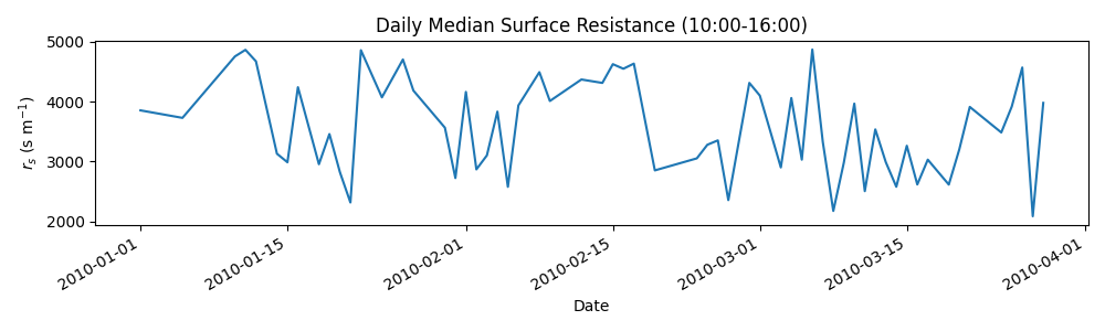
3.2.10. Surface Resistance Analysis#

Examine how surface resistance varies with environmental conditions.

ser_rs = df_results["RS"]

# Daily median resistance (filter extreme values)
df_rs_daily = ser_rs.between_time("10:00", "16:00").resample("1D").median()
df_rs_daily = df_rs_daily[df_rs_daily < 5000]  # Filter outliers (high in winter)

if not df_rs_daily.dropna().empty:
    fig, ax = plt.subplots(figsize=(10, 3))
    df_rs_daily.plot(ax=ax)
    ax.set_xlabel("Date")
    ax.set_ylabel(r"$r_s$ (s m$^{-1}$)")
    ax.set_title("Daily Median Surface Resistance (10:00-16:00)")
    plt.tight_layout()
else:
    print("No valid surface resistance data for this period")

Daily Median Surface Resistance (10:00-16:00)

3.2.11. Summary#

This tutorial demonstrated how to configure SUEWS for a custom site using the OOP API:

Create simulation: from_sample_data() for defaults
Configure site: update_config() with nested dictionary structure
Load forcing: update_forcing() with automatic resampling
Run simulation: run() returns SUEWSOutput object

Key concepts:

update_config() accepts nested dicts: {"sites": {0: {"properties": {...}}}}
Forcing data is automatically resampled to match model.control.tstep
Data cleaning requires extracting .df, modifying, then passing back

Next steps:

tutorial_03_impact_studies - Sensitivity analysis and scenario modelling

Total running time of the script: (0 minutes 30.814 seconds)

Gallery generated by Sphinx-Gallery